Thermal Conduction in Distributed Parameter Systems

Overview

This project analyzes thermal conduction in distributed parameter systems, specifically focusing on coupled heat transfer between spherical masses connected by a conducting rod. The study combines lumped and distributed parameter approaches to model complex thermal dynamics with both conduction and convection heat transfer mechanisms.

Approach

• Distributed Parameter Modeling: Applied hyperbolic PDE solutions for heat conduction in finite rods
• Lumped System Analysis: Coupled ordinary differential equations for spherical thermal masses
• Symbolic Mathematics: Used MATLAB symbolic toolbox for exact Laplace domain solutions
• Numerical Integration: ODE45 solver for time-domain temperature evolution
• Validation Methods: Compared multiple solution approaches for consistency verification

System Configuration

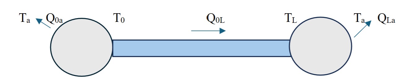
The thermal system consists of two iron spheres connected by a conducting rod with the following specifications:

% Material properties (Iron)
Cp = 452;      % Specific heat (J/kg-K)
K = 83.5;      % Thermal conductivity (W/m-K)
den = 7870;    % Density (kg/m³)

% Geometry
D = 0.5;       % Sphere diameter (m)
L = 2;         % Rod length (m)
As = pi*D^2;   % Sphere surface area (m²)
Ar = 0.25*pi*D^2;  % Rod cross-sectional area (m²)
vol = (pi*D^3)/6;   % Sphere volume (m³)
M = vol*den;        % Sphere mass (kg)

% Convection parameters
Ta = 273;      % Ambient temperature (K)
h = 25;        % Heat transfer coefficient (W/m²-K)

Distributed Parameter Solution

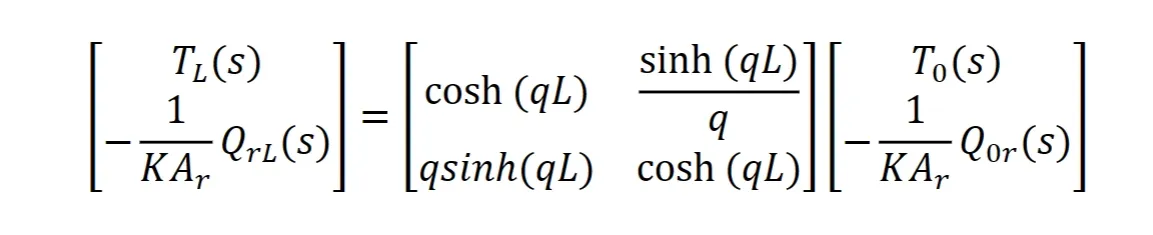
The rod temperature distribution follows the heat equation with boundary conditions imposed by the spherical thermal masses:

% Distributed parameter solution for rod temperature
% U(x,s) = A*cosh(q*x) + B*sinh(q*x)
% where q = sqrt(s/(K*Ar)) and boundary conditions couple to spheres

% Verification of temperature distribution
syms x s q real;
Delta_U = @(x,s) A*cosh(q*x) + B*sinh(q*x);

% Temperature derivative for heat flux
Delta_Ux = @(x,s) A*q*sinh(q*x) + B*q*cosh(q*x);

% Boundary conditions at x=0 and x=L
% -K*Ar*(dU/dx)|_{x=0} = Q_{0r}(s)
% -K*Ar*(dU/dx)|_{x=L} = Q_{rL}(s)

Coupled Energy Balance Equations

The system dynamics are governed by energy balances for each sphere:

% Energy balance for sphere at x=0
% dT0/dt = [-h*As*(T0-Ta) - (K*Ar/L)*(T0-TL)] / (Cp*M)

% Energy balance for sphere at x=L  
% dTL/dt = [(K*Ar/L)*(T0-TL) - h*As*(TL-Ta)] / (Cp*M)

% System of ODEs
odefun = @(t, x) [
    (-h*As*(x(1)-Ta) - (K*Ar/L)*(x(1)-x(2))) / (Cp*M);
    ((K*Ar/L)*(x(1)-x(2)) - h*As*(x(2)-Ta)) / (Cp*M)
];

% Initial conditions
T0_initial = 200;  % Initial temperature at x=0 (K)
TL_initial = 400;  % Initial temperature at x=L (K)
x0 = [T0_initial; TL_initial];

Symbolic Laplace Domain Analysis

Advanced symbolic mathematics enabled exact transfer function derivation:

% Define symbolic variables for Laplace analysis
syms s TLa Q0r real;
syms a b c real;  % Distributed parameter terms
% a = cosh(qL), b = sinh(qL)/q, c = q*sinh(qL)

% Laplace domain equations
% T0(s) = a*TL(s) - (b/(K*Ar))*Q0r(s)
T0 = a*TLa - (b/(K*Ar))*Q0r;

% Energy balance equations in Laplace domain
eq1 = Cp*M*(s*T0 - T0_0) + h*As*(T0 - Ta/s) + Q0r == 0;
eq2 = Cp*M*(s*TLa - TL_0) - (QrL - h*As*(TLa - Ta/s)) == 0;

% Solve symbolically for TL(s)
sol = solve([eq1, eq2], [TLa, Q0r]);
TLa_sol = simplify(sol.TLa);

Temperature Evolution Results

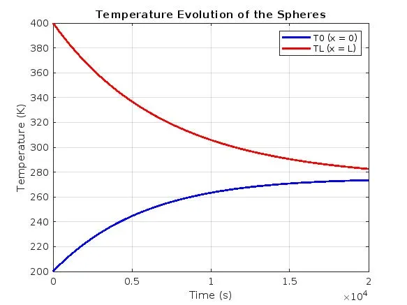
Numerical simulation over 20,000 seconds revealed the thermal dynamics:

% Solve ODEs using ode45
tspan = [0 20000];  % 20,000 second simulation
[t, x] = ode45(odefun, tspan, x0);

% Extract temperature profiles
T0 = x(:, 1);  % Temperature at x=0
TL = x(:, 2);  % Temperature at x=L

% Plot temperature evolution
figure;
plot(t, T0, 'b-', 'LineWidth', 2, 'DisplayName', 'T0 (x = 0)');
hold on;
plot(t, TL, 'r-', 'LineWidth', 2, 'DisplayName', 'TL (x = L)');
xlabel('Time (s)');
ylabel('Temperature (K)');
title('Temperature Evolution of the Spheres');
legend('show');
grid on;

Heat Transfer Rate Analysis

The analysis included computation of heat transfer rates throughout the system:

% Conduction heat transfer in rod
Q0L = (K*Ar/L)*(T0 - TL);

% Convection heat transfer at spheres
Q0a = h*As*(T0 - Ta);  % Sphere at x=0
QLa = h*As*(TL - Ta);  % Sphere at x=L

% Energy conservation verification
% Rate of energy storage = Conduction - Convection

Results

The comprehensive thermal analysis provided significant insights:

System Dynamics:

• Thermal Time Constants: Multiple time scales governing sphere cooling and rod equilibration
• Heat Transfer Coupling: Strong thermal coupling between spheres through conductive rod
• Convergence Behavior: Both spheres asymptotically approach ambient temperature

Engineering Applications:

• Thermal Management: Framework applicable to heat sink design and thermal control systems
• Material Processing: Understanding of cooling rates for metallurgical applications
• HVAC Systems: Distributed parameter modeling for building thermal analysis
• Electronics Cooling: Coupled conduction-convection for component thermal design

Methodology Validation:

• Symbolic-Numeric Agreement: Exact symbolic solutions validated through numerical integration
• Energy Conservation: Heat transfer rates satisfy conservation principles
• Physical Consistency: Temperature evolution matches expected thermal behavior

This work demonstrates sophisticated heat transfer analysis combining analytical and numerical methods, providing a robust framework for thermal system design and optimization in engineering applications.