Suspension System Estimation
Developed a method to estimate suspension system parameters using experimental data and modeling.
Overview
This project focuses on estimating the parameters of a suspension system by leveraging experimental data and advanced modeling techniques.
Using MATLAB, I processed real-world measurements from a csv file to identify system dynamics, fit transfer functions, and analyze damping and frequency characteristics. The workflow demonstrates my ability to combine data analysis, signal processing, and control theory to extract meaningful insights from physical systems. This approach is valuable for engineering applications where accurate modeling and parameter estimation are critical for design and optimization.
Approach
- Data Acquisition: Collected experimental data from a suspension system.
- Signal Processing: Used MATLAB to analyze the input (shake table) and output (mass) signals.
- System Identification: Applied frequency response and curve fitting to estimate the transfer function.
- Parameter Extraction: Analyzed poles, damping, and frequency characteristics.
MATLAB Code
SuspensionData=readmatrix('SuspData.xlsx');
t=SuspensionData(:,1);r=SuspensionData(:,2);y=SuspensionData(:,3);
figure(1)
plot(t,r,'r',t,y,'k:','LineWidth',3);
xlabel('Time, s','FontSize',18,'FontWeight','bold')
ylabel('Displacement, m','FontSize',18,'FontWeight','bold')
legend('shake table','mass',"fontsize",18,"FontWeight","bold")
title('Student ID 1001876127','FontSize',18,'FontWeight','bold')
xlim([0 2])
grid
[Gxx,Gyy,Gxy,Mag,Phase,CohF,FRF,f]=csdf(2^13,r,y,0.001,3);
[Num,Den]=frfcfit(FRF,f,14,4);
Y_s=tf(Num,Den)
damp(Y_s);

%output
Y_s =

    -0.5521 s^3 + 22.38 s^2 + 2.231e04 s + 2.86e05
  --------------------------------------------------
  s^4 + 26.62 s^3 + 2353 s^2 + 3.074e04 s + 2.843e05

Continuous-time transfer function.
Model Properties

         Pole              Damping       Frequency      Time Constant
                                       (rad/seconds)      (seconds)

 -7.12e+00 + 9.43e+00i     6.03e-01       1.18e+01         1.40e-01
 -7.12e+00 - 9.43e+00i     6.03e-01       1.18e+01         1.40e-01
 -6.19e+00 + 4.47e+01i     1.37e-01       4.51e+01         1.62e-01
 -6.19e+00 - 4.47e+01i     1.37e-01       4.51e+01         1.62e-01
>>
Results
The identified transfer function and its properties provide insight into the dynamic behavior of the suspension system, including damping ratios and natural frequencies. This enables better design and optimization for real-world engineering applications.
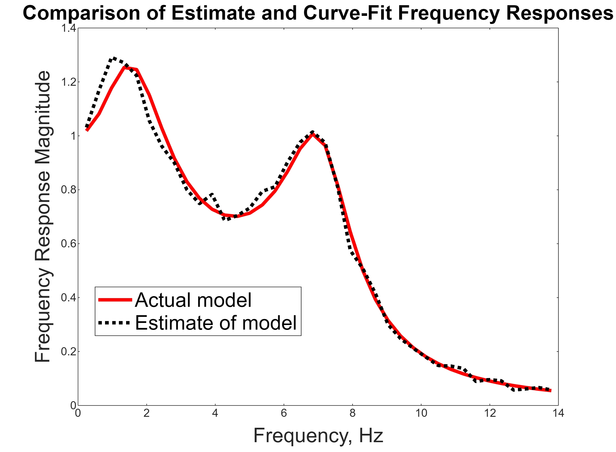
1. Frequency Response Plots
Magnitude Plot
- Shows how the suspension system reacts to different road frequencies.
- Peaks: Frequencies where the car will vibrate or “bounce” the most (possible discomfort).
- Dips: Frequencies that are suppressed by the suspension.
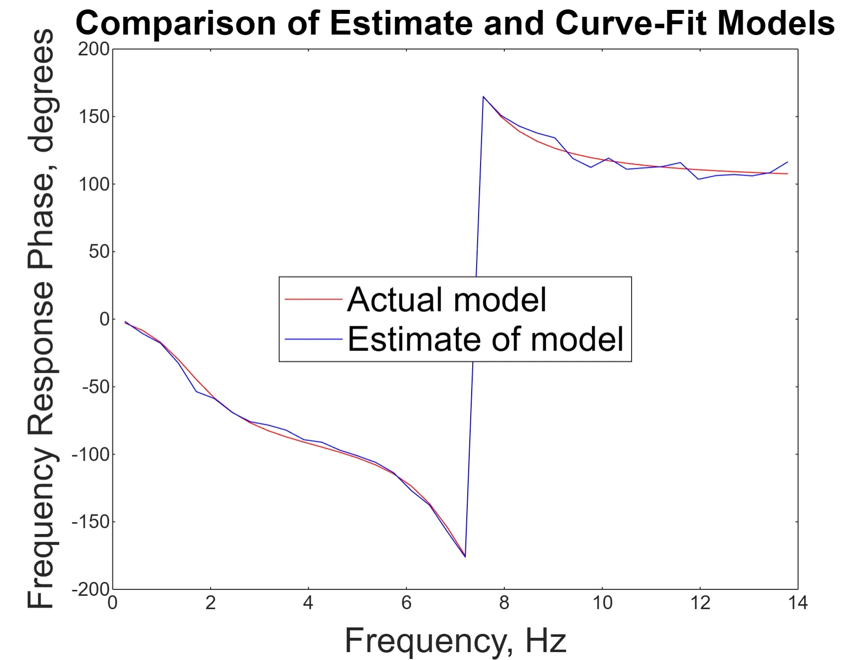
Phase Plot
- Shows how the timing (phase) of the car body’s movement lags behind the road input.
- Sudden phase changes: Align with resonance frequencies (system’s natural response points).
Practical Use
- Compare model and real-world system to ensure the model predicts actual behavior.
- Validate suspension tuning before moving to costly prototypes.
2. Pole, Damping, Frequency, and Time Constant Table
| Pole | Damping | Frequency (rad/s) | Time Constant (s) | Practical Meaning |
|---|---|---|---|---|
| -7.12 + 9.43i, -7.12 - 9.43i | 0.603 | 11.8 | 0.14 | Main ride mode: Moderate damping (good comfort), natural bounce of the car |
| -6.19 + 44.7i, -6.19 - 44.7i | 0.137 | 45.1 | 0.162 | High-frequency mode: Low damping (may cause “buzz” or harshness if excited) |
What These Results Mean Practically
Comfort
- The first mode (~1.88 Hz or 11.8 rad/s) is in the typical “ride comfort” range.
- The damping ratio (0.603) suggests the car won’t be too bouncy or too stiff—likely a comfortable ride.
Noise/Harshness
- The second mode (~7.18 Hz or 45.1 rad/s) has a much lower damping ratio (0.137), which means if this mode is excited (e.g., sharp road inputs), it could lead to a harsh or noisy ride.
- This frequency might correspond to vibrations felt in the seat or steering wheel.
Design/Improvement
- If the low-damping high-frequency mode is a problem, engineers may increase damping or adjust mass/spring properties to suppress it.
- Matching the estimated and actual frequency responses means the model is reliable for further tuning.